Data Science Class 7 – Logistic Regression

In this class, we would build a logistic regression model.

We would cover the following topics:

1. The Logistic Regression Model
2. Import the Necessary Modules
3. Generate the Dataset
4. Visualize the Data Using ScatterPlot
5. Perform Logistic Regression
6. View the Metrics
7. Create the Sigmoid Plot

Note: Logistic Regression is a Classification algorithm and hence discussed under Classification

1. The Logistic Regression Model

You already learnt from Class 6 (Introduction to Classification) that given values of x, we need to determine the class, y.  In other words, we aim to find the function that relates x and y. In the case of linear regression, this function is of the form:

y = f(x) = b0 + b1x

However, in the case of logistic regression, the output must be 0 or 1. So to achieve this, we need two things:

• a function that would alway return a value between 0 and 1
• a threshold to round off this output to either a 0 or a 1

To solve the first issue, we would model the outputs as probabilities. For example, we have a dataset of bank customers with credit card debt and we want to predict which customers will default. The input variable would be the balance on the customers account. The function will be something like this

Pr(default = Yes | balance)

This is shortened as p(balance) and will always give a value between 0 and 1 (since probability values are in range of 0 and 1)

The solve the second issue we have to choose a threshold. For example, we may predict default = Yes for customers whose p(balance) > 0.5.

Before we go into the practical, I would just want you to know about the logistic function which is give below.

Ok, let’s now go into the fun part!

2. Import the Necessary Modules

All the necessary modules we need are given below. I’m sure by now, you know what each of them are used for:

from sklearn.datasets import make_classification
from matplotlib import pyplot as plt
from sklearn.linear_model import LogisticRegression
from sklearn.model_selection import train_test_split
from sklearn.metrics import confusion_matrix
import pandas as pd

3. Generate the Dataset

We generate a dataset here using the make_classification function from sklearn.datasets.

# Generate and dataset for Logistic Regression
x, y = make_classification(
    n_samples=100,
    n_features=1,
    n_classes=2,
    n_clusters_per_class=1,
    flip_y=0.03,
    n_informative=1,
    n_redundant=0,
    n_repeated=0
)

You can actually change the number of samples to something more.

4. Visualize the Data Using ScatterPlot

Let’s now just do a scatter plot of this data. So we see why linear regression would not work quite well

# Create a scatter plot
plt.scatter(x, y, c=y, cmap='rainbow')
plt.title('Scatter Plot of Logistic Regression')
plt.grid( linestyle='--')
plt.show()

The output is given below:

5. Perform Logistic Regression

To perform the logistic regression, we would take two steps:

• split the dataset into train and test datasets
• create a logistic regression object
• fit the logistic regression object through the train data set

These three steps are given below in Python code

# Split the dataset into training and test dataset
x_train, x_test, y_train, y_test = train_test_split(x, y, random_state=1)

# Create a Logistic Regression Object, perform Logistic Regression
log_reg = LogisticRegression()
log_reg.fit(x_train, y_train)

6. View the Metrics

We are interested in view the following metrics

• the logistic regression coefficients
• the predicted values
• the confusion matrix

# Show to Coeficient and Intercept
print(log_reg.coef_)
print(log_reg.intercept_)

# Perform prediction using the test dataset
y_pred = log_reg.predict(x_test)

# Show the Confusion Matrix
confusion_matrix(y_test, y_pred)

The confusion matrix is explained as given below:

# True positive: (top-left) (We predicted a positive result and it was positive)
# True negative: (lower-right) (We predicted a negative result and it was negative)
# False positive:(top-right) (We predicted a positive result and it was negative)
# False negative: (lower-left) (We predicted a negative result and it was positive)

You can also use the following code to check that a data value belongs to either class 0 or 1 (No or Yes).

# Check the actual probability that a data point belongs to a class
lr.predict_proba(x_test)

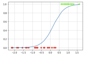
7. Create the Sigmoid Plot

The code below creates a sigmoid plot of our dataset

# Create and sort a dataframe containing our data
df = pd.DataFrame({'x': x_test[:,0], 'y': y_test})
df = df.sort_values(by='x')


# The expit function, also known as the logistic function, is defined as expit(x) = 1/(1+exp(-x)).
# It is the inverse of the logit function.
from scipy.special import expit
sigmoid_function = expit(df['x'] * log_reg.coef_[0][0] + log_reg.intercept_[0]).ravel()
plt.plot(df['x'], sigmoid_function)
plt.scatter(df['x'], df['y'], c=df['y'], cmap='prism')
plt.show()

The output of this code is given below:

This wraps up our class on Logistic Regression. I strongly recommend you watch the video for a clearer explanation.