Simple Linear Regression in Machine Learning (A Simple Tutorial)

In this tutorial we would cover Simple Linear Regression in a very easy-to-understand way. We are assuming you don’t have much knowledge of Machine Learning and maybe a little knowledge of statistics.

We would examine the following topics:

1. Introduction to Simple Linear Regression
2. What is  β₀ and β₁
3. Estimating Regression Coefficients β₀ and β₁
4. Method of Least Squares

 

 

1.  Introduction to Simple Linear Regression

Simple linear regression lives up to its name: it is a very straightforward approach for predicting a quantitative response Y on the basis of a single predictor variable X. It assumes that there is approximately a linear relationship between X and Y

Consider the dataset in table 1.0. The table shows the amount of Sales for  a given amount spent on advertising.

Year	Adverts (X)	Sales (Y)
2008	$60	$1500
2009	$75	$2200
2010	$77	$3500
2011	$89	$4230
2012	$93	$5500
2014	$101	$5910
2015	$104	????
2018	$110	????

Table 1.0: Yearly Sales Values for Adverts

The goal of simple linear regression is to predict the Sales for given advert. In order words, we want to predict the response Y(dependent variable), based on the predictor variable X (independent variable).

In Simple Linear Regression, we make an assumption that there exists a linear relationship between the two variable.  The easiest way to make this prediction is to find the function y = f(x) that relates the two variable. This we can do by:

• plot the table on a graph
• draw the line
• find the equation of the line

The equation of a line is given by

y = mx + c

But in the language of regression we write it as

Y ≈ β₀ +β₁X

Note that we did not use equal sign (=). The sign ≈ is a regression operator that says that Y is “modeled as” and not Y is equal to.

 

 

2. What are β₀ and β₁?

These are called the regression coefficients, model coefficients or model parameters which are unknown.

• β₁ represents the slope of the  model
• β₀ represents the intercept term

In Machine learning, the training data is used to determine values that are close to β₀ and β₁ but not exactly. If we call the coefficients produced by the training β₀‘ and β₁‘, then we can predict the values of future sales using the formula:

y’ = β₁‘ +β₀‘x

The ‘ in the variables indicate the the values are estimates of the unknown parameters.

 

 

3. Estimating the Model Coefficients

To estimate the coefficients β₀ and β₁, we need to use the data we have. In the Table 1.0, you can see that we have 6 known data points and 2 unknown points. We can represent out dataset as:

(x₁,y₁), (x₂,y₂), . . . , (x_n, y_n)

where n = 6.

For our dataset, (x₁,y₁) = (60, 1500). (x₂, y₂) = ( 75, 2200) and so on.

If we use the method of plotting the graph and making the line pass through each of the datapoint, we would get the exact values of β₁ and β₀. We would use our training data set to  obtain estimate β₀‘ and β₁‘

So if we want to make an estimate for the value of sales for 2018, we would, apply the coefficients such that:

y’ = β₀‘ +β₁‘ * 110

The objective is to find the estimated coefficietns  β₀‘ and β₁‘ that is a close to  β₀ and β₁ as possible.  The difference between our estimated value and the real values is an error term which needs to be minimized. The method we are going to use to do this is called the Least Squares approach. Let’s see how it works

 

 

4. The Least Squares Approach

Let’s assume we find the value of   y_i‘ = β₀‘ + β₁‘x_i for the ith observation.

Then we can calculate the error e_i = y_i – y_i‘. This value is called the ith residual. That is, the difference between the actual value of y and the estimated value of y predicted by the model.

Calculating the residual sum of squares (simply square the residual) for all the data, we have

Residual Sum of Squares (RSS) = e₁² + e₂² + . . . + e_n².

Knowing that e_i = y_i – y_i‘ and  y_i‘ = β₀‘ +β₁‘x_i,

We can write the summation as:

RSS = (y₁ – β₀‘ – β₁‘x1)² + (y₂ – β₀‘ – β₁‘x2)² + . . . + (y_n – β₀‘ – β₁‘x_n)²

The Method of Least Squares chooses β₀‘ and β₁‘ so as to minimize the RSS.

The values of β₀‘  and β₁‘ that would make the RSS minimum is given by the following equations:

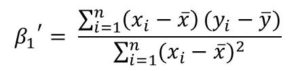
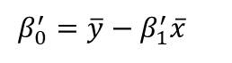
The formulas above are actually very simple to understand.

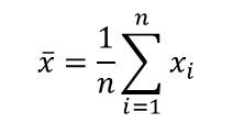
x̄ is the sample mean of the x dataset   and is given by:

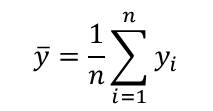
 is the sample mean for the y dataset and is given by:

In the next Tutorial on the regression series, we would take a real dataset, calculate these values, calculate the regression coefficients and actually use the the coefficients to predict missing values in the dataset.

Or I could give this as an exercise: Use the formulas to predict the missing values in Table 1.0.

Do leave a comment if this have been informative for you.